RF Power Support Engineering

How to Specify Power, Bias, Protection and Thermal Interfaces for an RF Power Module

An engineering workflow for turning RF operating modes into DC rail, current transient, ripple, sequencing, protection, heat-load, cooling-interface and acceptance requirements without confusing catalog ratings with delivered system performance.

Published: Jul 15, 2026
Reading time: 14 min

Unattended RF power module support verification setup with isolated DC converter, bias controller, current measurement, amplifier baseplate and controlled cooling hardware

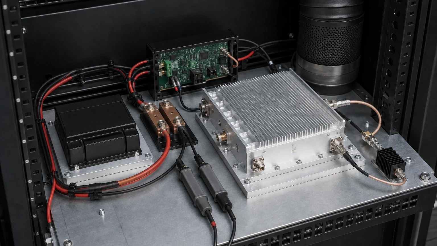
Define one electrical-and-thermal operating envelope

A usable RF module support specification ties supply, bias, protection and heat rejection to the same operating states and reference boundaries. It states what voltage reaches the module during startup, standby, RF drive, pulse bursts and faults; how current and ripple are measured; which rail or control changes first; where temperature is limited; and which tests prove the assembled path. Separate catalog ratings leave gaps between the source, wiring, converter, bias network, RF device and cooler.

Keep the article boundary on support hardware

This workflow owns the DC source and conversion path, bias generation and sequencing, enable logic, protection and telemetry, module heat flow, cooling interface and the acceptance evidence that joins them. It applies to RF power modules, externally biased amplifiers, remote front ends and test fixtures where electrical or thermal conditions can change gain, linearity, noise, efficiency or reliability.

It does not select RF output power, frequency coverage, gain, modulation linearity or antenna mismatch requirements. Those inputs arrive from the amplifier and system design. It also does not convert a generic family page into a stock claim: project voltage, current, cooling and protection details still require an approved model record or a reviewed custom requirement.

Freeze operating states before choosing hardware

List off, storage, startup, standby, receive-only, low-power alignment, full RF drive, pulse burst, calibration, shutdown and each credible fault state. For every state, record the active rails, RF drive, expected duration, repetition, ambient or coolant condition and whether the system must continue, derate, mute or latch off. A single nominal operating point cannot represent a transmitter that alternates between idle and high crest-factor bursts.

The state table becomes the common reference for supply sizing, sequencing, protection and thermal analysis. If the current profile is defined for one waveform while cooling is calculated for another, neither conclusion is valid. Include simultaneous channels, startup into discharged capacitors, recovery after a trip and the worst permitted mismatch or output loading when those conditions affect DC input or heat.

Specify voltage at the module terminals, not only at the source

State the source or bus minimum, nominal and maximum values, including startup ramp, surge, brownout, hold-up and reverse-polarity conditions. Then allocate connector, fuse, filter, switch, cable and return-path drop so the RF module still sees its permitted rail range. Remote sense can correct steady wiring loss, but it can also create instability or overshoot if the sense path opens or the load is disconnected.

Separate input-bus tolerance from converter regulation and module tolerance. A 28 V nameplate does not answer whether the module accepts 24 V during a transient, 30 V during charging, or a local overshoot after a long cable. Declare the measurement point, bandwidth and probe connection for every voltage limit, and define whether the limit applies before, during or after a load step.

Size current from the driven profile and fault envelope

Record quiescent, standby, average driven, pulse-on, peak and fault current at each rail. Include pulse width, duty cycle, burst length, repetition rate and crest factor. The continuous source, converter, wiring and connector are often governed by average and RMS heating, while local capacitance, current limiting and voltage droop are governed by the edge rate and peak step. Using RF output watts as DC supply watts ignores efficiency and auxiliary loads.

Measure current with the intended RF drive, bias, load, temperature and control mode. If the supply enters current limit during a burst, the observed PA compression or spectral regrowth may be a power-path failure rather than an RF design limit. State whether the supply must support the peak directly, share it with local energy storage, or deliberately limit it, and define the allowed rail excursion in each case.

Turn the load step into droop, recovery and stability limits

Define the current-step amplitude, rise and fall time, repetition, initial load and allowed voltage overshoot or undershoot. A converter has finite loop bandwidth, so output capacitance and its ESR and ESL support the first part of a fast step. More capacitance can reduce droop but may slow startup, increase inrush or destabilize a converter whose compensation was not designed for that load network.

Specify recovery time and ringing, not only the peak deviation. Test at minimum and maximum input, cold and hot conditions, and the wiring and filter configuration used in the assembly. A bench supply with short leads can pass while a remote rack source with an input filter oscillates or produces a deeper droop. If hot plug is required, it must be explicitly supported and verified; it cannot be inferred from wide input range.

Allocate ripple and noise against RF degradation

Power-supply ripple can modulate an RF carrier into discrete spurs, while broadband and low-frequency rail noise can add AM or PM noise. The sensitivity depends on the amplifier, rail, frequency, bias point and RF operating condition. Therefore a generic millivolt number is not enough: state the spectral band, detector or FFT method, bandwidth, probe loop, load state and RF metric that must remain inside its budget.

Start from the allowed RF spur or phase-noise contribution and characterize supply-to-RF sensitivity where the risk is material. Allocate margin, then derive a rail-noise limit across the relevant offset frequencies. Switching frequency, harmonics, beat products and control-mode transitions deserve explicit checks. An LDO can reduce noise but adds dissipation; a switching converter can improve efficiency but may require filtering, layout control and verified stability under the real load.

Write the complete power-up, RF-enable and power-down sequence

For externally biased depletion-mode or GaN stages, the required gate and drain order must come from the approved device or module data. A common safe pattern applies the required gate condition before drain voltage, confirms a bounded quiescent drain current, and removes drain before releasing the gate on shutdown. Enhancement-mode or internally biased modules may use a different sequence, so technology names must not replace the actual interface specification.

Give voltage thresholds, delays, ramp rates, current windows and timeout actions for each step. Define when RF drive may be applied and when it must be removed relative to bias and drain control. Include discharge behavior and restart after an interrupted sequence. A sequence diagram that shows only nominal timing but omits power-good validity, stuck controls and partial rails is not a protection specification.

Make every protection function observable and deterministic

Define overvoltage, undervoltage, overcurrent, short circuit, reverse polarity, overtemperature, missing cooling, reflected-power or external interlock conditions as applicable. For each one, state the sensing point, threshold, tolerance, debounce or blanking time, action, safe-state sequence, latch or retry behavior and the conditions required to reset. The threshold must be coordinated with normal pulse current and startup inrush so protection does not create nuisance trips.

Telemetry should identify what is actually measured: source current is not necessarily drain current, and heatsink temperature is not junction temperature. Specify sample rate, accuracy, update latency, alarm state and behavior if the sensor or communication link fails. Acceptance should inject faults or simulate them at the defined boundary rather than merely checking that a status bit can toggle.

Calculate heat from DC input and RF output under the same condition

For a power stage, heat is based on dissipated power, not RF output alone. At a steady condition, use measured DC input to the relevant stage minus delivered RF output, then add losses from drivers, converters, control electronics and other heat sources that cross the same thermal boundary. For pulsed operation, decide whether the thermal mass responds to average dissipation, pulse energy or a transient junction limit; the answer depends on pulse duration and the published transient thermal model.

Use efficiency measured at the actual frequency, output level, waveform, temperature and mismatch state. A best-case saturated efficiency figure will underpredict heat during backed-off linear operation. State the maximum allowed junction, case or baseplate temperature and keep those references distinct. Top-surface temperature is not a substitute for the specified thermal reference unless a correlation method has been validated.

Close the path from module baseplate to ambient or coolant

Define the heat-spreader or cold-plate material, contact area, flatness, surface finish, interface material, thickness, compression, fastener pattern and torque. Allocate thermal resistance across module, interface, spreader, sink and fluid or air path. Air cooling also needs inlet temperature, altitude, flow rate, pressure drop, recirculation and fan-fault behavior; liquid cooling needs fluid composition, inlet range, flow, pressure drop, material compatibility, leak detection and condensation control.

The drawing must show keep-out zones and where temperature is sensed. A large heatsink with poor contact can perform worse than a smaller, well-coupled one. When the module relies on chassis conduction, loose mounting or thick interface material can invalidate the rating. Verify the assembled thermal path at the worst credible heat load, not a detached component on an ideal laboratory cold plate.

Design one acceptance matrix that joins electrical, RF and thermal evidence

Measure source and module-terminal voltage, rail current, enable and bias timing, fault response and declared temperatures while the RF module operates in the approved states. Where supply quality affects RF behavior, correlate rail waveform or spectrum with output power, gain, modulation quality, spurs or phase noise. Keep the same reference planes, probes, cable lengths, cooling setup and firmware state across comparison units.

Retain raw waveforms or data, instrument and probe bandwidth, calibration or verification state, sample location, ambient or coolant conditions, RF stimulus, load state, serial numbers, drawing and firmware revisions, thresholds, uncertainty and deviations. A pass/fail screenshot without these conditions cannot support a replacement unit, a production limit or a later root-cause investigation.

Decision matrix for the support interface

Boundary	Requirement to freeze	Reject when
Operating states	Rail, RF drive, duration, repetition, environment and required response for each state	Only one nominal point is supplied
Voltage	Bus range, module-terminal range, drop, surge, ramp, hold-up and measurement point	A source nameplate is treated as delivered voltage
Current	Quiescent, average, RMS, pulse, peak, inrush and fault profiles	RF output power is used as the DC requirement
Transient	Step size and edge, allowable droop or overshoot, recovery, ringing and stability	Only steady regulation is specified
Ripple and noise	Spectrum, bandwidth, probe method, load state and allocated RF impact	One unconditioned millivolt value is quoted
Sequence	Thresholds, order, delays, current window, RF enable, shutdown and restart	Technology assumptions replace module instructions
Protection	Sense point, tolerance, response time, safe action, latch or retry and reset	Protection cannot distinguish normal pulses from faults
Thermal	Heat load, temperature reference, interface stack, airflow or coolant and fault case	RF output watts or heatsink size is used as proof
Evidence	Coupled electrical, RF and thermal test data with conditions and revision traceability	Only catalog curves or isolated bench checks exist

Worked example: translate RF output into current, heat and local energy storage

Assume a 50 W CW RF stage delivers 50 W at 45% drain efficiency from a 28 V rail, while 5 W of driver and control dissipation crosses the same baseplate boundary. The PA drain input is 50 / 0.45 = 111.1 W, or about 3.97 A at 28 V. The total heat to remove is 111.1 - 50 + 5 = 66.1 W. If the allowed baseplate-to-coolant rise is 35°C, the allocated assembled thermal resistance cannot exceed 35 / 66.1 = 0.53°C/W. These numbers illustrate the method and are not a rating for a published LCRF product.

Now assume the rail must supply an additional 4 A for 100 µs before the converter loop responds, with no more than 0.5 V ideal capacitive droop. The first-order capacitance is C = ΔI × Δt / ΔV = 800 µF, before ESR, ESL, tolerance, bias derating, wiring and control-loop effects. The design must then be tested for overshoot, recovery and stability. This calculation rules out choosing a supply only from average watts, but it does not replace measured load-step data.

The four boundaries that must remain connected

Text-free engineering schematic showing source conversion, bias and transient control, RF power module protection and thermal rejection as one verification boundary — The diagram separates source and conversion, rail and bias dynamics, protected RF load, and heat rejection while keeping their control and measurement paths connected. Localized captions carry the explanation; the asset contains no language-dependent text.

Acceptance sequence from source bus to cooled RF operation

Approve the operating-state matrix, RF stimulus, load or mismatch state and environmental boundary.
Freeze the source, converter, filters, wiring, return, connector, remote-sense and local capacitance configuration.
Instrument source and module-terminal voltage, each relevant current, enable and bias controls, fault lines and declared temperature points.
Verify startup, standby, RF enable, full drive, pulse or burst behavior, controlled shutdown and restart after interruption.
Apply the specified load steps at minimum and maximum input and temperature; record droop, overshoot, ringing and recovery.
Measure ripple and noise with the declared bandwidth and probe method, then check associated RF spurs or noise where allocated.
Inject or simulate each required fault and confirm threshold, latency, safe-state sequence, latch or retry and telemetry.
Run the worst credible heat condition with the final thermal interface, airflow or coolant and verify steady and transient temperatures.
Repeat critical electrical and RF checks after thermal equilibrium and after fault recovery.
Archive raw data, uncertainty, calibration state, serials, configuration photos without people, drawings, firmware and deviations.

Common failures hidden by separate component ratings

Sizing the supply from RF output power instead of driven DC input and auxiliaries
Ignoring wiring and return-path drop at the module terminals
Using average current for a pulse or burst source with inadequate local energy storage
Adding output capacitance without checking converter startup and loop stability
Quoting ripple without bandwidth, spectrum, probe loop or RF operating condition
Applying drain voltage before the required gate condition or RF drive before bias is stable
Setting current protection below normal pulse demand or above a safe device boundary
Treating heatsink temperature, case temperature and junction temperature as interchangeable
Calculating heat from RF output watts or best-case efficiency
Validating a cooler with an ideal cold plate that is not present in the delivered assembly
Testing fault status without injecting the real electrical or thermal condition
Accepting screenshots without raw data, reference planes or configuration traceability

Use published product data as evidence, not as a universal design rule

The current LCRF record for the MXD-M isolated DC-DC converter documents 30 W to 150 W options, several input and output ranges, typical 85% to 86% efficiency, remote control, output overcurrent and short-circuit protection, and case-mounted cooling. Its dynamic-response entry is 4% of output voltage, while ripple and noise are stated as 1% typical with a 20 MHz test bandwidth. The record also states that hot plug is not supported. These conditions are more useful than a bare wattage because they identify boundaries that an assembly must preserve.

The same record includes an output derating curve, recommends chassis contact or an external heatsink, and distinguishes model-specific input ranges and protections. Those facts apply only to the approved MXD-M configurations and test conditions. They must not be projected onto PA supplies, bias networks, liquid coolers or unpublished voltage combinations. Use the linked product page for the current model record and submit project-specific rail and thermal requirements for review.

RF power, bias and thermal RFQ inputs

RF module or device record, frequency and required RF operating states
Source bus minimum, nominal, maximum, surge, brownout, hold-up and grounding boundary
Required rails and tolerances at the module terminals, including wiring and filter drop
Quiescent, standby, average, RMS, pulse-on, peak, inrush and fault current profiles
Pulse width, duty cycle, burst structure, repetition, crest factor and simultaneous channels
Allowed voltage droop, overshoot, ringing and recovery for specified load steps
Ripple and noise spectrum, measurement bandwidth and allowed RF spur or noise contribution
Bias and enable thresholds, order, delays, ramp rates, current windows and shutdown sequence
Protection thresholds, tolerances, response times, latch or retry, reset and telemetry behavior
DC input, RF output and auxiliary dissipation at worst frequency, waveform, temperature and load
Maximum junction, case or baseplate temperature and the exact temperature reference
Thermal interface drawing, flatness, material, thickness, torque and sensor location
Air inlet or coolant temperature, flow, pressure, altitude, recirculation and loss-of-cooling case
Required acceptance waveforms, RF correlations, environmental points, raw data and traceability

Continue the same engineering decision

Related FAQ

How should an RF power amplifier supply be sized for peak current, duty cycle and load transients?

Size the continuous source, converter, wiring and connector for measured driven average and RMS current, then size local energy storage and transient response for the pulse-on or burst step. Record quiescent, average, peak, edge rate, pulse width, duty cycle, burst length, inrush and fault current at the intended voltage, RF drive, load and temperature; RF output watts alone are not a DC requirement.

Reject a supply that meets average watts but enters current limit, exceeds allowed rail droop, rings, recovers too slowly or becomes unstable with the final cable, input filter and output capacitance. State whether the source or local capacitor supplies the first part of the step, and coordinate protection so normal pulses do not trip while unsafe current is still interrupted within the required time.

As a first check, a 4 A step lasting 100 µs with 0.5 V allowed ideal droop needs C = ΔIΔt/ΔV = 800 µF before ESR, ESL, tolerance and converter response. Supply the current waveform, rail limits, wiring, capacitance, input range and temperature so the final design can be verified by load-step and RF tests rather than by wattage comparison alone.

How much power-supply ripple and noise can an RF amplifier tolerate?

An RF amplifier does not have one universal acceptable ripple value. Specify rail noise versus frequency, measurement bandwidth and probe method, then relate it to allowable carrier spurs, AM noise or phase noise at the relevant frequency, output level, bias and modulation state. A millivolt RMS figure without spectrum and test conditions cannot be applied safely.

Reject a regulator or filter when switching fundamentals, harmonics, beat products, burst-mode transitions or low-frequency noise exceed the allocated RF contribution, even if total RMS ripple looks small. Where risk is material, inject known rail modulation or compare controlled supplies to characterize the supply-to-RF transfer, then retain margin for layout, grounding and unit variation.

Provide the RF limit, offset-frequency range, rail, bias point, load state, regulator mode, filter, grounding and measurement setup. LDO post-regulation can lower noise but adds heat; switching conversion can reduce dissipation but needs verified filtering and stability. Selection is a measured tradeoff, not an automatic preference for either topology.

What bias sequencing and protection are required for an RF power amplifier?

The required sequence comes from the approved RF device or module record. Externally biased depletion-mode and many GaN stages commonly require the gate condition before drain voltage, a verified quiescent drain-current window, RF enable only after bias is stable, and drain removal before the gate is released; internally biased or enhancement-mode modules may require a different order.

Write voltage thresholds, ramp rates, delays, timeouts, current limits and power-good validity for startup and shutdown. Reject a controller that cannot handle missing or partial rails, stuck enables, excessive drain current, overtemperature, loss of cooling or an interrupted sequence. Define safe state, latch or retry behavior, discharge and reset conditions instead of relying on a nominal timing sketch.

Provide the device bias instructions, gate and drain ranges, target quiescent current, allowed RF-enable point, normal pulse-current envelope and fault limits. Acceptance should capture the real gate, drain, enable, current and fault waveforms and inject representative faults; toggling a status bit alone does not prove device protection.

What thermal-interface data are needed before selecting air or liquid cooling for an RF power module?

Begin with heat dissipated under the worst credible RF operating state: measured DC input minus delivered RF output, plus auxiliary losses that cross the same thermal boundary. State the maximum junction, case or baseplate temperature and where it is measured; RF output watts, top-surface temperature and a generic heatsink rating are not interchangeable thermal inputs.

For either air or liquid cooling, define contact area, flatness, surface, interface material and thickness, fastener pattern and torque. Air systems also need inlet temperature, altitude, flow, pressure and recirculation; liquid systems need fluid, inlet range, flow, pressure drop, compatibility, leak and condensation controls. Reject a design that passes only on an ideal cold plate or at room ambient.

Provide heat versus operating mode, allowable temperature rise, mechanical drawing, sensor location, environment and fault response. For example, 66 W through a 35°C baseplate-to-coolant budget allows at most 0.53°C/W for the assembled path. Verify that allocation at thermal equilibrium and during relevant transients with the delivered interface and cooling hardware.

Engineering inquiry

Share your RF requirement

Share the product, operating requirements and project context. Our engineering team will route your request to the right specialist.